
INTRODUCTION
Idiopathic sudden sensorineural hearing loss (ISSNHL) refers to rapid-onset hearing loss of more than 30 dB at least three consecutive frequencies within 72 hours [1-3]. This disease is a common otologic emergency, with an estimated incidence and prevalence of 10–20 per 100,000 person years and 5–160 per 100,000 person years, respectively [1,2]. Although the exact etiology and pathogenesis of ISSNHL remain ambiguous, viral disease and vascular compromise have been strongly suggested as causes. In addition, retrocochlear lesions such as vestibular schwannoma and strokes should be considered [3,4]. Because ISSNHL is diagnosed only by describing the symptoms of hearing loss, regardless of the cause, treatment methods are inevitably diverse. Despite the lack of standardized treatment guidelines for ISSNHL, steroid therapy—including systemic, intratympanic, or both in combination—is widely accepted as the most effective option [3-5]. Numerous prognostic factors have also been identified in recent years, including age, duration from onset to treatment, initial hearing level, vertigo/dizziness, smoking, alcohol use, and blood test parameters [4,6]. Based on these diverse prognostic factors, the ability of various models to prognosticate ISSNHL has been studied. In addition to traditional statistical techniques such as multiple-regression and logistic-regression (LR) models, researchers have attempted to predict the prognosis of ISSNHL using Bayesian cure-rate models [7-10]. Recently, some researchers have applied various machine learning techniques [1,11].
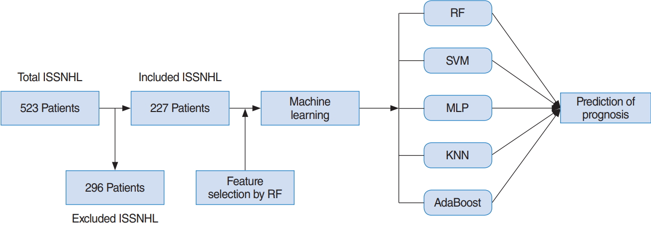
In a previous report, several machine learning models, including LR, support vector machines (SVMs), multilayer perceptrons (MLPs), and deep-belief networks (DBN), were applied to predict the hearing outcomes of sudden sensorineural hearing loss [1]. The sample size of that study was 1,220, and 149 variables were analyzed. For variable selection, the study utilized the results of univariate statistics (P<0.05) and expert knowledge [1]. In the present study, the effectiveness of five potential machine learning models (K-nearest neighbor [KNN], random forest [RF], SVM, adaptive boosting [AdaBoost], and MLP) for predicting hearing recovery in ISSNHL patients was investigated. The sample size of our study was 227, and 32 variables were. Furthermore, we conducted variable selection based on an RF algorithm and medical domain knowledge. This study aimed to assess the effectiveness of predicting hearing recovery in patients with ISSNHL after 1 month of treatment using the five aforementioned machine learning models.
MATERIALS AND METHODS
Study population
We performed a retrospective study of in-patients admitted to Korea University Ansan Hospital for treatment of ISSNHL. We inspected 523 unilateral ISSNHL patients enrolled from January 2010 to October 2017. In this study, we analyzed the hearing improvement after 1 month of treatment for 227 patients with all variables analyzed. The diagnostic criteria for ISSNHL included sudden hearing loss (30 dB or more) for at least three contiguous frequencies over 3 days. We evaluated their entire medical history, laboratory examinations, and audiologic results. Exclusion criteria were: (1) bilateral ISSNHL, (2) conductive hearing loss >10 dB, (3) vestibular schwannoma, and (4) data with missing values.
All included patients were hospitalized and treated using systemic steroids (e.g., methylprednisolone 64 mg, tapering for 14 days or dexamethasone 5 mg intravenously three times/day for 5 days and then tapered over 7 days) with/without intratympanic dexamethasone injection (ITDI; 1–4 times). During the initial hospital day, each patient underwent a pure-tone audiogram, which was then repeated posttreatment 1 month later. We measured hearing thresholds at 0.125, 0.25, 0.5, 1, 2, 3, 4, and 8 kHz. Siegel’s criteria were classified as follows: (1) complete recovery included final hearing levels better than 25 dB, (2) partial recovery was >15-dB gain and final hearing levels between 25 and 45 dB, (3) slight recovery was >15-dB gain and final hearing poorer than 45 dB, and (4) no improvement was <15-dB gain, or final hearing poorer than 75 dB [12].
In this study, patients with hearing gains of at least “partial recovery” based on Siegel’s criteria, i.e., complete recovery and partial recovery were considered to be the recovery group. Patients under the “slight recovery” classification according to Siegel’s criteria were regarded as the no-recovery group. This study obtained the approval of the Institutional Review Board at Korea University Ansan Hospital (IRB. No. 2018AS0044). The overall procedure of this study is shown in Fig. 1.
Original variables and variable selection
The original number of variables was 32 (31 predictors and 1 response), as extracted from demographic data, medical records, inner-ear symptoms, pure-tone audiometry, and laboratory data. Hearing improvements after 1 month of treatment were based on Siegel’s criteria, which considered patients under complete recovery and partial recovery as the recovery group (positive in classification). The others were the no-recovery group (negative in classification). In detail, there were 11 independent categorical variables: sex, smoking status, hypertension, diabetes mellitus, hyperlipidemia, stroke, chronic kidney disease, myocardial infarction/angina, dizziness, tinnitus, and timing of ITDI. The categorical variables were mostly binary variables with “yes/no” values. The timing of ITDI was classified into three conditions: never (0), 0–12 days from onset (1), and more than 13 days from onset (2). The smoking status was divided into three conditions: never (0), current (1), and ex-smoker (2). Then, the timing of ITDI and smoking statuses were changed to binary variables having the same number of classes for KNN and MLP. Additionally, there were 20 independent continuous variables, including age at time of diagnosis, pack-year for smoking, systolic blood pressure, diastolic blood pressure, duration from onset to treatment (day), hemoglobulin, erythrocyte sedimentation rate, activated partial thromboplastin time (aPTT), blood urea nitrogen (BUN), creatinine (Cr), initial hearing by frequency (0.125, 0.25, 0.5, 1, 2, 3, 4, and 8 KHz), prothrombin time (PT) result (second), and PT result (%). All continuous variables were scaled into a range between 0 and 1 via min–max scaling to fairly compare the five machine learning algorithms. Because KNN and MLP are very sensitive to scaling, it was necessary to scale the data. In this study, we used variable selection to improve the predictive performance for hearing recovery.
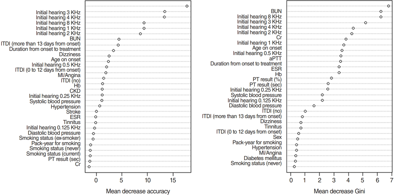
For variable selection using a RF, mean decrease accuracy and Gini were used [13]. The greater the decrease in the accuracy of RF after a permutation of a specific variable, the more important that variable [13]. Therefore, variables with a large mean decrease in accuracy were more important when predicting hearing outcome. However, RF is based on Gini, which is a splitting criterion. When a decrease in Gini is significant, the parent node is split into two child nodes. Therefore, to evaluate the importance of a specific variable, the mean decrease of Gini can be calculated for all decision trees in an RF. The greater the mean decrease of Gini, the more important the variable when predicting a hearing outcome [13]. When training an RF with 1,000 trees and six variables at random, the variable importance score is calculated according to the mean decrease accuracy and mean decrease Gini, as shown in Fig. 2.
The top five variables, excluding initial hearing by frequency (0.125, 0.25, 0.5, 1, 2, 3, 4, and 8 KHz) in each criterion, are included, and all values for initial hearing by frequency are included. As a result, the 15 variables, including initial hearing by frequency, BUN result, timing of ITDI, duration from onset to treatment (days), dizziness, age of onset, Cr result, and aPTT result are shown in Fig. 2. Additionally, original variables and selected variables were applied to the five machine learning models to compare the effect on the performance of the two sets of variables in predicting hearing outcome after 1 month of treatment.
Statistical analysis methods and model development
A total of 523 enrolled ISSNHL patients were admitted between January 2010 to October 2017. The number of missing data points for each variable varied, especially for recovery status, which had the most missing data because of follow-up losses. Therefore, we implemented a complete deletion method using a rule in which patients having at least one missing value in variables were excluded. As a result, we obtained 227 patients in total, 106 for the recovery group and 121 for the no-recovery group. All statistical hypothesis tests were two-sided. Statistical tests were implemented using R v.3.5.0 (The R Foundation, Vienna, Austria). In this study, to inspect the differences among groups with recovery and those with no recovery, two-sample t-tests were used for the continuous random variables and chi-square or Fisher’s exact tests for the categorical random variables. The difference was considered statistically significant at a two-tailed P-value of less than 0.05. According to our results, initial hearing by frequency (0.125, 0.25, 0.5, 1, 2, 3, 4, and 8 KHz), age on onset, BUN result, hypertension, dizziness, and the timing of ITDI, turned out to be statistically significantly different between the recovery and norecovery groups under a significance level of 0.05. The statistical test results are listed in Table 1.
We split the data (n=227) into training and test sets. The ratio of the sizes of the training set and test set was 7 to 3, respectively, which resulted in a training set with a sample size of 158 and a test set with a sample size of 69. We then evaluated five different machine learning models and implemented three-fold cross validation on the training set to determine the hyperparameters for each model to optimize the validation accuracy by calculating the accuracy of the validation set. Therefore, we selected the optimal hyperparameters for each model that maximized the accuracy of the validation set. Then, we evaluated our model using the selected hyperparameters on the test set. The accuracy of the test set for each model is listed in Table 2. The training set was randomly divided into three subsets that were similar in size, among which, two were used to train each model, and one was used as the validation subset to verify model efficiency.
In this study, several model evaluation criteria such as accuracy, recall (sensitivity), and F-score were utilized for machine learning techniques and to compare the prediction performance of the five models. The machine learning models are summarized in detail below.
K-nearest neighbor
KNN is based on the assumption that the observations within a dataset generally exist closely to other observations having similar attributes. If the observations have a classification label, the label of an unclassified observation can be identified by considering the class of its nearest neighbors. KNN finds the k-nearest observations to the test observation and determines its class by majority voting (Fig. 3). While implementing three-fold cross validation, the hyperparameter, K, was tuned until the training subset produced the highest accuracy. The optimal parameter was then applied to the test set, which did not affect the training or cross-validation procedures [14].
Random forest
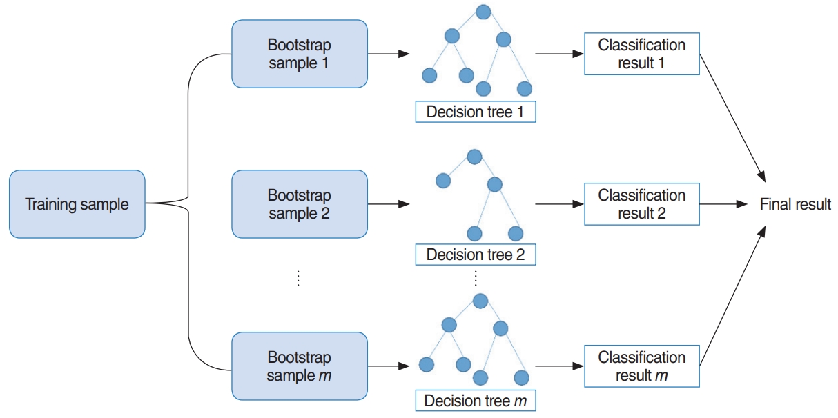
RF uses bootstrap sampling to create new training samples. The new training samples are then used to train m different decision trees. As a result, this algorithm aggregates prediction results from m different decision trees, usually via majority voting [13]. The overall model is shown in Fig. 4. Additionally, we determined two parameters using three-fold cross validation, which are the number of decision trees to train and the number of predictors to sample from the original variables.
Support vector machine
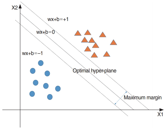
SVM is used to establish a separating hyperplane having a maximum margin. This model leads to a good generalization ability and can classify nonlinear data more easily than a linear classifier such as logistic regression. The concept of SVM is shown in Fig. 5. To classify nonlinear data, a kernel function such as a Gaussian kernel is required [15]. In this study, a Gaussian kernel function was used to classify the nonlinear data. Furthermore, we determined two hyperparameters for SVM, which are the regularization parameter (C) and spread-parameter sigma (σ) to optimize three-fold cross-validation accuracy.
AdaBoost
Boosting is a machine learning approach based on the concept of creating high-accuracy models by combining many low-accuracy ones, called weak learners. The AdaBoost algorithm by Freund is the most widely used boosting algorithm [16]. It is a very accurate classifier that uses a decision tree as the base model, i.e., the weak learner. It is used to train a multiple decision trees based on weight-updated and aggregated results from classifier models. The overall AdaBoost algorithm is shown in Fig. 6. In this study, the AdaBoost model was trained using the “fast Adaboost” package in R ver. 3.5.0 (R Foundation for Statistical Computing, Vienna, Austria). Additionally, we determined two parameters, the number of decision trees and maximum depth, using three-fold cross validation accuracy.
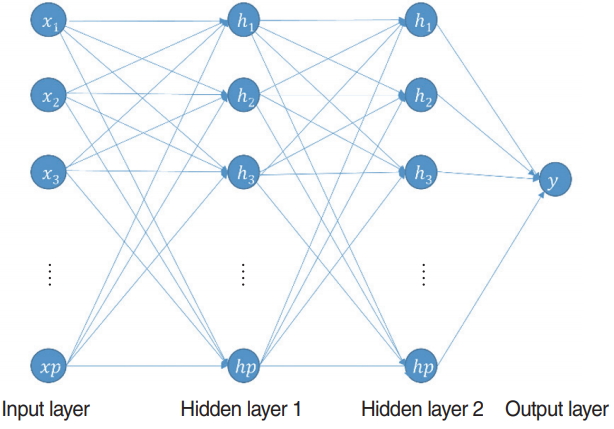
Multilayer perceptron
The MLP is a feed-forward neural network that uses the backpropagation method for training. This model can classify nonlinear data. Generally, MLP comprises one input layer, one or more hidden layers, and one output layer. The overall architecture of this model is shown in Fig. 7. It can be used both for classification and for regression problems. In this study, we used it as a binary classifier to classify in-patients after 1 month of treatment. The original and selected variables were utilized as input variables. Thus, they determined the number of input nodes. All nodes of each hidden layer were fully connected to the nodes of the previous layer. Because this study regarded a binary classification problem, the number of nodes of the output layer was one. This node represents the probability of hearing recovery after 1 month of treatment. We determined two hyperparameters, which are the number of hidden layers and its activation function. In addition, the learning rate was 0.1, number of epochs was 10,000, and batch size was 20. In this study, MLP was developed by adopting the “deepnet” package in R ver. 3.5.0.
RESULTS
Clinical characteristics of patients according to their recovery status
The study population consisted of 227 unilateral ISSNHL patients, including 121 who did not recover and 106 who recovered. There were 70 men and 157 women, with a mean and standard deviation (SD) age of 46.43±14.77 years and 51.3±99.65 years, respectively. The clinical characteristics of patients according to their recovery status are listed in Table 1.
Continuous and categorical random variables were presented as mean±SD and percentages, respectively. The clinical and demographic characteristics of the patients who did or did not recover were compared using the two-sample t-test for continuous random variables and the chi-square test or Fisher exact test for categorical random variables.
All statistical hypothesis tests were two-sided. Statistical tests were implemented using R ver. 3.5.0. A mean difference was considered to be statistically significant when the P-value was less than 0.05. Statistically significant differences were found between the recovery and no-recovery groups according to initial hearing by frequency (0.125, 0.25, 0.5, 1, 2, 3, 4, and 8 KHz), age at onset, BUN, hypertension, dizziness, and the timing of ITDI. The statistical test results are presented in Table 1.
Model performance results
The SVM model with selected variables was determined to be the best-performing prediction model (accuracy, 75.36%; F-score, 0.74), and the RF model with selected variables was the secondbest model (accuracy, 73.91%; F-score, 0.74). The accuracy of the RF model with the original variables was the same as that of the RF model with selected variables (accuracy, 73.91; F-score, 0.73). However, the prediction time for the test set (n=69) of the SVM model with selected variables was nearly zero (R.3.5.0, RAM 8 GB), while that of RF with selected variables was 0.01 s (R.3.5.0, RAM 8 GB). Thus, the SVM model with selected variables performed better than the RF model with selected variables, considering both accuracy and the computation time required for the classification under real clinical circumstances. To summarize, the SVM model with 31 predictors was the best model, whereas the second-best model was RF with 15 predictors (Table 2, Fig. 8). Additionally, the results of the training set are provided in Table 3 and Fig. 9.
DISCUSSION
In our analysis, the RF model with the original variables predicted the prognosis of ISSNHL. In a recent study, several machine learning models [1] were used to predict the hearing outcomes of ISSNHL patients. In that study [1], the accuracy of prediction of hearing outcomes was 67.45%–73.32% for LR, 68.14%–73.41% for SVM, 63.90%–74.03% for MLP, and 60.67%–77.58% for DBN. A total of 1,220 inpatients with ISSNHL were admitted between June 2008 and December 2015, and four-fold cross-validation was applied to the dataset. In contrast, our study included a total of 227 inpatients with ISSNHL between January 2010 and October 2017. Three-fold cross-validation was applied to the dataset. In our study, the accuracy of the prediction of hearing outcomes was 75.36% for SVM, 73.91% for RF, 72.46% for AdaBoost, 72.46% for MLP, and 65.22% for KNN. Thus, compared with the previous study, we trained a model with a similar generalization performance, but using a much smaller sample size. Furthermore, in another study, the accuracy of prediction of hearing outcomes was 76.6% for AdaBoost, 76.9% for RF, 81.9% for MLP, and 83.0% for SVM. In that study, 10-fold cross-validation was implemented, and the study population was 1,113 subjects from 17 factories [11]. To the best of our knowledge, our study is the first in Korea to compare the effectiveness of multiple machine learning models for predicting the prognosis of ISSNHL.
A limitation of this study is its small sample size (227 patients), compared to previous studies that included 1,220 patients [1] and 1,113 patients [11]. Furthermore, the number of predictors may not have been sufficient compared with that of a former study that used 149 potential predictors [1]. Machine learning performance depends on the sample size and number of predictors. As the sample size and number of predictors increase, the model performance is expected to improve. Therefore, further research with a larger sample size is needed.
In conclusion, the accuracy of predicting hearing outcomes was 75.36% for SVM, 73.91% for RF, 72.46% for MLP, 72.46% for AdaBoost, and 65.22% for KNN, which are comparable to those of a previous study with a sample size of 1,220 [1]. Therefore, given a higher sample size and more predictors, we can expect better prediction performance with our model. Moreover, the SVM model with selected variables (accuracy, 75.36%) was found to be the most helpful for clinicians to predict the hearing prognosis of patients diagnosed with ISSNHL.